Learning Vector Quantisation (LVQ) is a supervised version of vector quantisation, similar to Selforganising Maps (SOM) based on work of LINDE et al. [4, 13, 18], GRAY [33] and KOHONEN (see [21, 25] for a comprehensive overview). It can be applied to pattern recognition, multi-class classification and data compression tasks, e.g. speech recognition, image processing or customer classification. As supervised method, LVQ uses known target output classifications for each input pattern of the form .
LVQ algorithms do not approximate density functions of class samples like Vector Quantisation or Probabilistic Neural Networks do, but directly define class boundaries based on prototypes, a nearest-neighbour rule and a winner-takes-it-all paradigm. The main idea is to cover the input space of samples with ‘codebook vectors’ (CVs), each representing a region labelled with a class. A CV can be seen as a prototype of a class member, localized in the centre of a class or decision region (‘Voronoї cell’) in the input space. As a result, the space is partitioned by a ‘Voronoї net’ of hyperplanes perpendicular to the linking line of two CVs (mid-planes of the lines forming the ‘Delaunay net’; see Fig. 4). A class can be represented by an arbitrarily number of CVs, but one CV represents one class only.

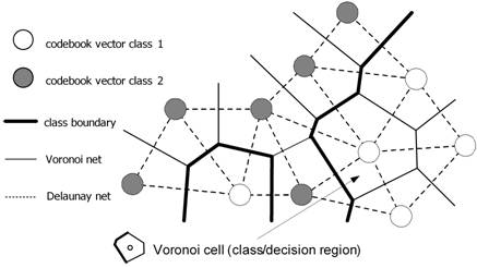
Fig. 4: Tessellation of input space into decision/class regions by codebook vectors
represented as neurons positioned in a two-dimensional feature space.

In terms of neural networks a LVQ is a feedforward net with one hidden layer of neurons, fully connected with the input layer. A CV can be seen as a hidden neuron (‘Kohonen neuron’) or a weight vector of the weights between all input neurons and the regarded Kohonen neuron respectively (see Fig.5).

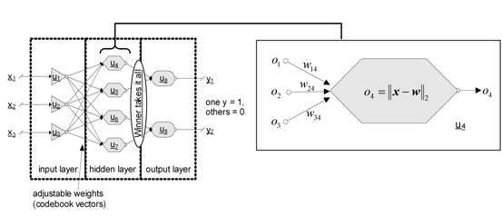
Fig. 5: LVQ architecture: one hidden layer with Kohonen neurons, adjustable weights between input and hidden layer and a winner takes it all mechanism

Learning means modifying the weights in accordance with adapting rules and, therefore, changing the position of a CV in the input space. Since class boundaries are built piecewise-linearly as segments of the mid-planes between CVs of neighbouring classes, the class boundaries are adjusted during the learning process. The tessellation induced by the set of CVs is optimal if all data within one cell indeed belong to the same class. Classification after learning is based on a presented sample’s vicinity to the CVs: the classifier assigns the same class label to all samples that fall into the same tessellation – the label of the cell’s prototype (the CV nearest to the sample).
The core of the heuristics is based on a distance function – usually the Euclidean distance is used – for comparison between an input vector and the class representatives. The distance expresses the degree of similarity between presented input vector and CVs. Small distance corresponds with a high degree of similarity and a higher probability for the presented vector to be a member of the class represented by the nearest CV. Therefore, the definition of class boundaries by LVQ is strongly dependent on the distance function, the start positions of CVs, their adjustment rules and the pre-selection of distinctive input features.
The basic LVQ algorithm LVQ1 rewards correct classifications by moving the CV towards a presented input vector, whereas incorrect classifications are punished by moving the CV in opposite direction. The magnitudes of these weight adjustments are controlled by a learning rate which can be lowered over time in order to get finer movements in a later learning phase. Improved versions of LVQ1 are KOHONEN’s OLVQ1 with different learning rates for each CV in order to get faster convergence and LVQ2, LVQ2.1 and LVQ3. Since LVQ1 tends to push CVs away from Bayes decision surfaces, it can be expected to get a better approximation of the Bayes rule by pairwise adjustments of two CVs belonging to adjacent classes. Therefore, in LVQ2 adaptation only occurs in regions with cases of misclassification in order to get finer and better class boundaries. LVQ2.1 allows adaptation for correctly classifying CVs, too, and LVQ3 leads to even more weight adjusting operations due to less restrictive adaptation rules. All these algorithms are intended to be applied as extension to previously used (O)LVQ1 (KOHONEN recommends an initial use of OLVQ1 and continuation by LVQ1, LVQ2.1 or LVQ3 with a low initial learning rate). For a comprehensive overview and also details of heuristic learning algorithms of LVQ, readers are referred to standard ANN literature, e.g. [42] or [50]. More detailed information can be found in the above mentioned work of KOHONEN, or for specialized topics, e.g., in [11]. A good overview of statistical and neural approaches to pattern classification is given by [48] or [51]. Besides the above mentioned standard algorithms from KOHONEN, several extensions from various authors are suggested in literature, e.g. LVQ with conscience [34], Learning/Linear Vector Classification (LVC) [45], Dynamic LVQ (DLVQ) [46] or Distinction Sensitive LVQ (DSLVQ) [6]. In [47] LVQ algorithms are discussed and combined with genetic algorithms in order to select and weight useful input features automatically by weighted distances. Newer developments are LVQ4-algorithms with promising performance and results [8].
The accuracy of classification and, therefore, generalisation and the learning speed depend on several factors. Basically the developer of a LVQ has to prepare a learning schedule, a plan which LVQ-algorithm(s) – LVQ1, OLVQ, LVQ2.1 etc. – should be used with which values for the main parameters at different training phases. Also, the number of CVs for each class must be decided in order to reach high classification accuracy and generalisation while avoiding under- or overfitting. Additionally, the rule for stopping the learning process as well as the initialisation method (e.g. random values, values of randomly selected samples) determine the results.

Home | Neural Associations | Neural Applications | Neural Data Sources | Neural Community | Neural Contacts | Neural Publications | Neural News&Events | Neural Software | Neural Tutorials | Neural Links | Forecasting Principles

©  2002-2005 BI³S-lab - Hamburg, Germany - All rights reserved - Questions, Comments and Enquiries via eMail -  [Impressum & Disclaimer]
The Knowledge Portal on Forecasting with Neural Networks @ www.neural-forecasting.com -